Turbulent Channel Flow SGS Model

Source

• Scripts: channel_flow_sim.py (simulation and data generation) and channel_flow_learning.py (training, inference, evaluation)
• Instructions: TCF.md in the repository
• Setup: the turbulent channel flow experiment of the PICT paper

This is the flagship learning experiment of the paper. A turbulent channel flow (TCF) at \(\text{Re}_\tau = 550\) runs on a coarse grid, where it cannot resolve the near-wall turbulence. A neural network learns to output a correcting force so that the statistics of the corrected low-resolution simulation match the DNS reference. No paired high-resolution data is used.

Streamwise velocity near the lower wall. Top: no SGS model and Smagorinsky. Bottom: the learned SGS model and the down-sampled high-resolution reference. (Franz et al. 2026, Fig. 14)

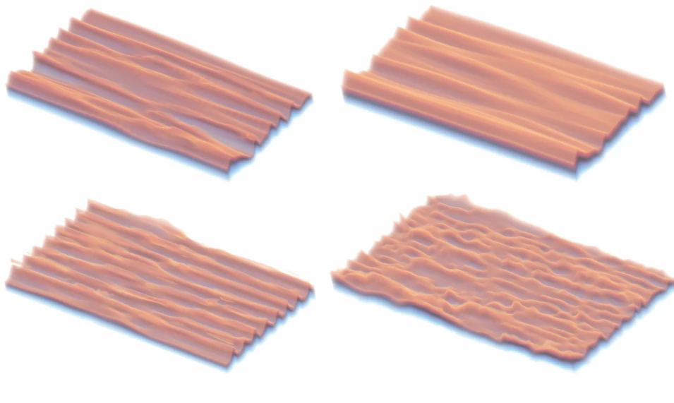
The setup

The channel is periodic in the streamwise (x) and spanwise (z) directions and has no-slip walls at \(\pm y\). Its size is \(2\pi\delta \times 2\delta \times \pi\delta\) with \(\delta = 1\). The grid is refined towards the walls. A dynamic forcing, recomputed in every step from the mean wall shear stress (see Velocity sources), drives the flow, so it does not lose energy:

Re_wall = 550
Re_center = TCF_tools.Re_wall_to_cl(Re_wall)     # center-line Reynolds number
u_wall = Re_wall / Re_center                     # friction velocity
viscosity = delta / Re_center

domain = PISOtorch.Domain(3, torch.tensor([viscosity], dtype=dtype), passiveScalarChannels=0,
                          name="ChannelDomain", device=cuda_device, dtype=dtype)
block = domain.CreateBlock(velocity=vel_init, vertexCoordinates=grid, name="ChannelBlock")
block.CloseBoundary("-y")                        # walls at -y and +y, periodic in x and z

The initial condition is a Reichardt mean profile perturbed with curl noise from the SimplexNoiseVariations extension (init_with_noise=True). Time is measured in eddy turnover times (ETT); TCF_tools converts between simulation time, ETT and wall units.

Step 1: reference statistics

Download the turbulence statistics from the Torroja channel database and place them in ./data/tcf_torroja/. The profiles Re*.prof are needed for training; the energy balances Re*.bal.* are optional and used in the evaluation:

./data/tcf_torroja/Re550.prof
./data/tcf_torroja/Re550.bal.ww
...
./data/tcf_torroja/Re180.prof
./data/tcf_torroja/Re180.bal.ww
...

Then compile the noise kernels:

cd extensions/noise
python setup_noise.py install

Step 2: simulate (optional validation)

channel_flow_sim.py runs the pure simulation. You can use it to validate PICT against the spectral references at high resolution, but this is expensive: a resolution of 256 can take several days. Skip it if you only want the SGS learning setup.

The script has two modes, selected by case at the top of its main section: "SIM" runs a simulation, and "EVAL" (the default) loads a finished run and evaluates its statistics. Set case = "SIM" to simulate. The main options are at the top of the case=="SIM" branch:

Option	Meaning
x, y	streamwise and wall-normal resolution (64 × 32 for training data, up to 256 × 128 for validation); the spanwise resolution is x/2
refinement_strength	wall refinement of the grid (3 for the 64-cell training data, 1 for high resolution)
target_ETT, iterations	simulated time and number of output iterations
adaptive_CFL	CFL number of the adaptive time stepping (0.1; higher values may laminarize the flow)
save_steps	save the state after every iteration (needed for training data)
load_run_id	continue from a previous run, identified by its time stamp
C_smag, use_van_driest	optional Smagorinsky SGS baseline

To reproduce the paper's results, run a noise-initialized warm-up of 20 ETT. Then load the warmed-up state and simulate another 20 ETT to accumulate the statistics. Output is written to ./test_runs/<time-stamp>_<name>/.

Step 3: create the training data

The statistics-based training still needs initial conditions from a developed low-resolution flow (64 × 32 × 32):

1. Run channel_flow_sim.py at this resolution for at least 10 ETT (better 20 ETT) to warm up.
2. Set save_steps = True and load_run_id = "<time-stamp>", and simulate at least another 20 ETT.

The time stamp, also called run id, consists of the first 13 characters of the run directory name.

Step 4: train

Training, inference and evaluation are all done by channel_flow_learning.py. Under ### DATA ###, select the initial conditions with load_run_id, load_frames = "<time-stamp>", <iterations>. The training is organized in intervals:

training_intervals = [
    {
        "opt_steps": 6000,   # optimization iterations
        "batch_size": 1,     # must be 1
        "pre_steps": 0,      # non-differentiable warm-up steps: int, interval [min, max], or callable
        "sim_steps": 12,     # differentiable steps after the warm-up
        "lr_net": 1e-4,
        "stats": 20,         # interval for recording training statistics
        "grads": 200,        # interval for gradient statistics (multiple of "stats")
        "eval": 2000,        # interval for running inference
    },
    # further intervals with randomized warm-up, e.g. "pre_steps": (0, 12), (0, 24), ...
]

In the script, only the first interval is active; the following ones are listed as comments and can be enabled. All intervals can be run at once, or one after another by loading the partially trained model with net_run_id = "<time-stamp>".

The model. CorrectionNet stacks seven 3D multi-block convolutions (filters 8, 64, 64, 32, 16, 8, 4; kernel size 3) with ReLU activations and a final 1×1 convolution to the 3 force components. In the paper, it receives the velocity and a wall-distance feature as input and has 198,931 parameters. The trainer can also output viscosities or velocity corrections instead of forces, and can use the cell volume as an additional input.

The loss. During the unrolled steps, the trainer accumulates differentiable online statistics: the mean velocity components (streamwise with weight 1, the other two with weight 0.5), the normal stresses \(\overline{u'u'}^+, \overline{v'v'}^+, \overline{w'w'}^+\) and the shear stress \(\overline{u'v'}^+\). It compares them in wall units to the Torroja profiles, both accumulated over the whole unroll and per frame (weight 0.5). A penalty on the forcing magnitude regularizes the output, the forcing is clamped to \([-2, 2]\), and a gradient modification steers it towards being divergence-free.

The schedule in the paper. Training has four phases. After each warm-up, 12 steps are backpropagated. The warm-up length is drawn from \([0,0]\), \([0,12]\), \([0,24]\) and \([0,96]\) steps in the four phases, for 6k + 3 × 20k iterations in total. The first training uses the fast approximate gradients without the backward linear solves. Fine-tuning with advection gradients helped only marginally.

Step 5: evaluate

Set eval_only = True and load the model with net_run_id = "<time-stamp>". Images and statistics plots are written to ./test_runs/<time-stamp>_<name>/ as before.

Results

Turbulence statistics with no SGS model (top), Smagorinsky (middle) and the learned model (bottom). The resulting Re_τ are 390, 452 and 548, against the target of 550. (Franz et al. 2026, Fig. 11)

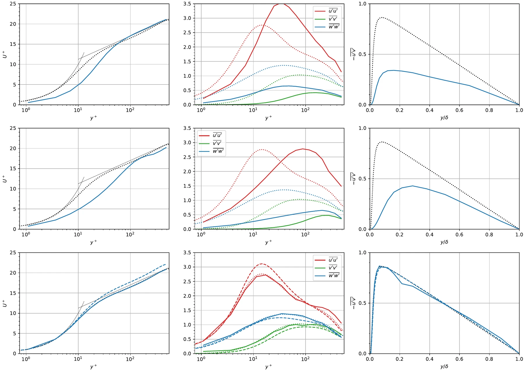
• The learned model matches the target statistics and also reproduces the turbulent energy budgets, which were not part of the loss.
• It remains stable for 20,000 steps, more than 180× the 108-step training horizon.
• With the learned model, PICT simulates 20 ETT in 223 s on a single GPU. That is about 40× faster than OpenFOAM at 192 × 96 × 96 on 32 CPU cores, and with a lower aggregated statistics error.

See Results from the Paper for more.