Buoyant Plume

Source

• Script: buoyancy_sample.py
• Run: python buoyancy_sample.py from the repository root

A plume of smoke rises in a closed box. The smoke is a passive scalar that is transported by the flow, and it acts back on the flow through a buoyancy force. PICT has no built-in buoyancy model: the coupling consists of three short callbacks. This makes the sample a template for any custom physics you want to inject into the PISO loop.

Smoke density of the buoyancy sample (64 × 128 cells, 200 iterations of 0.25 time units), simulated with PICT and rendered for this website.

Setup

• Closed box of 1 × 2 units with no-slip walls, 64 × 128 cells
• Viscosity \(2\cdot10^{-4}\), one passive scalar channel
• A random smoke source near the bottom center, refilled every step
• Upward force = 0.1 × smoke density
• 200 iterations of 0.25 time units with adaptive sub-steps

Smoke density at t = 6.25, 12.5, 25, 37.5 and 50.

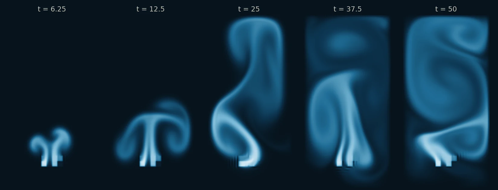
Domain with a passive scalar

dims = 2
x, y = 16 * 4, 32 * 4
grid = shapes.make_wall_refined_ortho_grid(x, y, corner_upper=(1, y / x), wall_refinement=[], base=1.10)
grid = grid.cuda().contiguous()

viscosity = torch.tensor([2e-4], dtype=dtype)
domain = PISOtorch.Domain(dims, viscosity, passiveScalarChannels=1, name="CavityDomain",
                          device=cuda_device, dtype=dtype)
block = domain.CreateBlock(vertexCoordinates=grid, name="CavityBlock")
block.CloseAllBoundaries()        # no-slip walls, scalar = 0 at the walls
domain.PrepareSolve()

Coupling through callbacks

The three callbacks run at different points of every PISO step (see Callbacks):

# a random source pattern: 4x4-cell patches near the bottom center
torch.manual_seed(83342666)
density_inflow = torch.rand((1, 1, y_base // 16, x_base // 4), dtype=dtype, device=cuda_device)
density_inflow = torch.repeat_interleave(density_inflow, res_factor, dim=2)
density_inflow = torch.repeat_interleave(density_inflow, res_factor, dim=3)
density_inflow = torch.nn.functional.pad(density_inflow, ((x - x // 4) // 2, (x - x // 4) // 2, 2 * y // 16, y - (3 * y // 16)))

def density_inflow_fn(domain, **kwargs):             # PRE: refill the source region
    block = domain.getBlock(0)
    block.setPassiveScalar(torch.maximum(block.passiveScalar, density_inflow).contiguous())
    domain.UpdateDomainData()

vel_src_velX_pad = torch.zeros_like(block.passiveScalar)
def buoyancy_fn(domain, time_step, **kwargs):        # PRE_VELOCITY_SETUP: smoke pushes the fluid up
    block = domain.getBlock(0)
    block.setVelocitySource(torch.cat([vel_src_velX_pad, block.passiveScalar * buoyancy_factor], dim=1))
    domain.UpdateDomainData()

def clamp_density(domain, **kwargs):                 # POST: no negative smoke
    block = domain.getBlock(0)
    block.setPassiveScalar(torch.clamp(block.passiveScalar, min=0).contiguous())
    domain.UpdateDomainData()

prep_fn = {
    "PRE": [density_inflow_fn],
    "PRE_VELOCITY_SETUP": [buoyancy_fn],
    "POST": clamp_density,
}

• PRE runs before the scalar is advected, so the source region is refilled first.
• PRE_VELOCITY_SETUP runs after the scalar has been advected and before the momentum system is assembled. The force is therefore computed from the current smoke field.
• POST clamps the small negative values that a central scheme can produce near sharp fronts.

Running the simulation

sim = PISOtorch_simulation.Simulation(domain=domain, prep_fn=prep_fn,
    substeps="ADAPTIVE", time_step=0.25, corrector_steps=2, pressure_tol=1e-5,
    advect_non_ortho_steps=1, pressure_non_ortho_steps=1, pressure_return_best_result=True,
    velocity_corrector="FD", non_orthogonal=False,
    log_interval=1, norm_vel=True, log_dir=run_dir, save_domain_name="domain", stop_fn=stop_handler)
sim.run(200)

python buoyancy_sample.py

The scalar images in the output directory (d_*.png) show the plume. The velocity (v_*.png) and velocity-source (vs_*.png) images show the flow it induces and the buoyancy force. The coupling consists of ordinary PyTorch operations in callbacks, so other source terms can be added in the same way.