Numerical Method

This page summarizes how PICT discretizes and solves the incompressible Navier–Stokes equations. Details, derivations and the backward pass are in the paper.

Governing equations

PICT solves the incompressible Navier–Stokes equations for the velocity \(\mathbf{u}\) and the kinematic pressure \(p\), with viscosity \(\nu\) and a source term \(\mathbf{S}\):

\[ \frac{\partial \mathbf{u}}{\partial t} + \nabla\cdot(\mathbf{u}\otimes\mathbf{u}) = -\nabla p + \nabla\cdot(\nu\nabla\mathbf{u}) + \mathbf{S}, \qquad \nabla\cdot\mathbf{u} = 0 . \]

Passive scalars obey the corresponding advection–diffusion equation, without a pressure term.

Finite volumes on curvilinear multi-block grids

PICT uses a cell-centered finite-volume method on collocated grids: velocity, pressure and scalars are all stored at the cell centers.

Each block is a structured grid. Its cells are mapped from a computational space \(\boldsymbol{\xi}\) with unit cell spacing to physical space \(\mathbf{x}\). For every cell, PICT precomputes from the vertex coordinates

• the metric matrix \(M = \partial\mathbf{x}/\partial\boldsymbol{\xi}\),
• its inverse \(T = M^{-1}\) with entries \(T_{ji} = \partial\xi_j/\partial x_i\),
• the Jacobian determinant \(J = \det M\), which is the cell volume.

The equations are solved in computational space. Fluxes through cell faces use the contravariant velocity and the diffusion operator uses the transformed Laplace coefficients:

\[ U^j = J\,T_{ji}\,u_i, \qquad \alpha_{jk} = J\,T_{ji}\,T_{ki}, \]

so that, for example, the transformed continuity equation reads \(\partial U^j/\partial\xi_j = 0\).

• Convection is written in conservative form and linearized: the face fluxes are linear averages of the contravariant velocities of the two adjacent cells, taken from the previous time step. The transported face values are linearly interpolated (central). No upwinding or flux limiters are used.
• Diffusion uses the transformed Laplacian. Its orthogonal part, with face coefficients \(\tfrac12(\nu_P\alpha_P + \nu_N\alpha_N)\), is implicit. On skewed meshes, the non-orthogonal cross terms \(\alpha_{jk}, j\neq k\) extend the stencil to the diagonal neighbors (9 cells in 2D, 19 in 3D). PICT keeps the contributions of the cell itself and its direct neighbors in the matrix and moves those of the diagonal neighbors to the right-hand side. These are updated in non-orthogonal corrector iterations, i.e. repeated solves (advect_non_ortho_steps, pressure_non_ortho_steps).
• Time integration is implicit (backward) Euler.
• Multi-block coupling. Blocks are connected conformingly, face to face with one-to-one cells, including permuted and flipped axes. The kernels look up neighbor cells across connections on the fly, and all blocks are assembled into one global sparse matrix per linear system, so the coupling between blocks is fully implicit.

The PISO algorithm

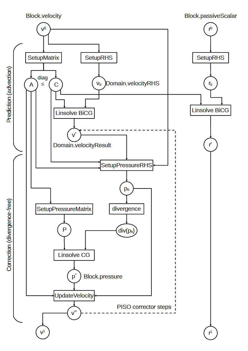
Pressure and velocity are coupled with the PISO algorithm (Issa, 1986). One predictor step is followed by two pressure-corrector steps by default.

1. Predictor. All velocity components are advected and diffused implicitly:

\[ C(\mathbf{u}^{n})\,\mathbf{u}^{*} = \frac{\mathbf{u}^{n}}{\Delta t} + \mathbf{S}, \]

where \(C\) contains the time derivative, the linearized advection and the diffusion. \(A = \operatorname{diag}(C)\) is its diagonal. The old pressure gradient is not included, so each corrector solves for the full pressure.

2. Correctors (corrector_steps, default 2). With the off-diagonal part \(H(\mathbf{u}) = \sum_{N} C_{PN}\mathbf{u}_N\):

\[ \mathbf{h} = A^{-1}\left(\frac{\mathbf{u}^{n}}{\Delta t} + \mathbf{S} - H(\mathbf{u}^{*})\right), \qquad \nabla\cdot\left(A^{-1}\nabla p\right) = \nabla\cdot\mathbf{h}, \qquad \mathbf{u}^{**} = \mathbf{h} - A^{-1}\nabla p . \]

The divergence of \(\mathbf{h}\) is computed from linearly interpolated face fluxes, and the pressure Laplacian is a compact face-based stencil with coefficients \(\tfrac12(\alpha_P/A_P + \alpha_N/A_N)\). With the default velocity_corrector="FD", the pressure gradient of the velocity correction is computed with central differences in computational space and transformed with the metrics, \((\nabla p)_i = \sum_j T_{ji}\,(p_{j+1}-p_{j-1})/2\). The next corrector starts from \(\mathbf{u}^{**}\). At prescribed boundaries, pressure has a zero normal gradient, and the mean pressure is removed after every solve.

3. The result of the last corrector is \(\mathbf{u}^{n+1}\). Passive scalars are advected at the beginning of each step with the same kind of implicit system.

One PISO step as a computational graph: prediction (advection–diffusion solve with BiCGStab) followed by the pressure correction (Poisson solve with CG and velocity update), repeated for each corrector step. Passive scalars are advected alongside. This graph is what the differentiable mode backpropagates through.

Linear solvers

All systems are assembled in CSR format across all blocks and solved on the GPU with custom CUDA code built on cuSPARSE and cuBLAS:

System	Matrix	Solver
advection–diffusion (velocity, scalars)	non-symmetric	BiCGStab, optionally with ILU(0) preconditioning (by default only as a fallback)
pressure	symmetric	CG

• The velocity components are solved as a batch of right-hand sides with the same matrix.
• Convergence is measured on the residual 2-norm divided by \(\sqrt{n}\) (the RMS of the residual vector, ConvergenceCriterion.NORM2_NORMALIZED), with default tolerances of 1e-5 (float32) and 1e-8 (float64). Both precisions are supported throughout. The paper's experiments use float32.
• The linear solves typically take 70–90% of the runtime.

Differentiability

The PISO operators above (matrix and right-hand-side setup, pressure setup, velocity correction) each have a hand-written CUDA backward kernel, as do the copies of the results back to the block fields. The linear solves are differentiated with the adjoint method, i.e. a solve with \(A^{\mathsf T}\). See Differentiable Simulation.

Mapping to the API

PISOtorch_simulation.Simulation composes these low-level operators of the PISOtorch module. You can call them yourself for custom algorithms:

Step	Operator	Writes
advection–diffusion matrix	SetupAdvectionMatrix(domain, dt, nonOrthoFlags, forPassiveScalar, passiveScalarChannel)	domain.C, domain.A
scalar / velocity right-hand side	SetupAdvectionScalar(...), SetupAdvectionVelocity(...)	domain.scalarRHS, domain.velocityRHS
linear solve	SolveLinear(A, RHS, x, maxIterations, tolerance, ..., useBiCG, ...)	x
pressure system	SetupPressureCorrection(...) (= SetupPressureMatrix + SetupPressureRHS)	domain.P, domain.pressureRHS (\(\mathbf{h}\)), domain.pressureRHSdiv (\(\nabla\cdot\mathbf{h}\))
velocity correction	CorrectVelocity(domain, dt, version)	domain.velocityResult
block ↔ global vectors	Copy{Velocity,Pressure,Scalar}Result{To,From}Blocks(domain)	block fields / global vectors

PISOtorch_diff provides autograd versions of these operators, with the linear solve as linear_solve_GPU.

Scope and limitations

As stated in the paper:

• PICT runs on a single GPU.
• Geometry is represented by structured multi-block grids. Building good meshes for complex geometries takes effort, and there are no gradients with respect to the mesh.
• The low-order discretization introduces numerical dissipation, so PICT is not intended as a replacement for high-fidelity turbulence solvers. Its strength is fast, differentiable simulation for learning and optimization.