Lid-Driven Cavity¤
Source
- Scripts:
minimal_lid_sample.py(2D) andminimal_lid_sample3D.py(3D) - Run:
python minimal_lid_sample.pyfrom the repository root
A square cavity with no-slip walls is driven by a lid that moves with constant velocity. This is the smallest complete PICT setup and the best place to start. It shows how to create a mesh, a domain and a block, how to set boundaries, and how to run a simulation with adaptive time stepping and output.
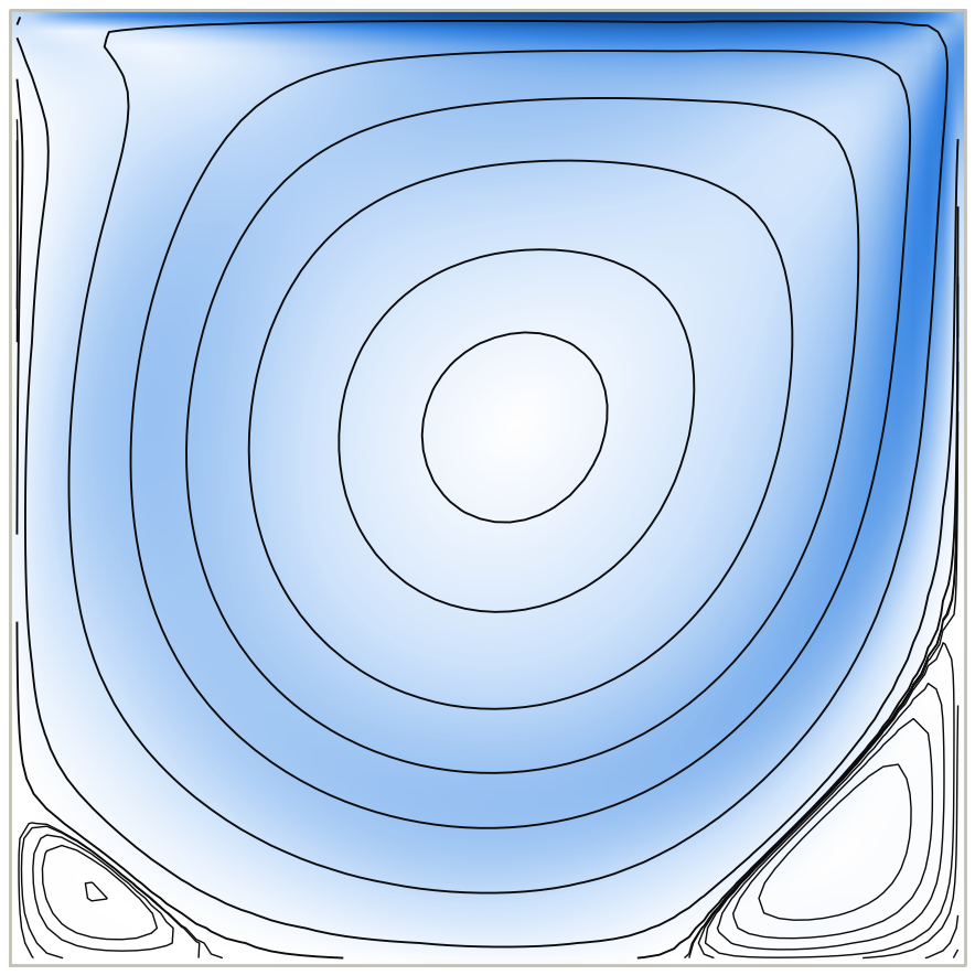
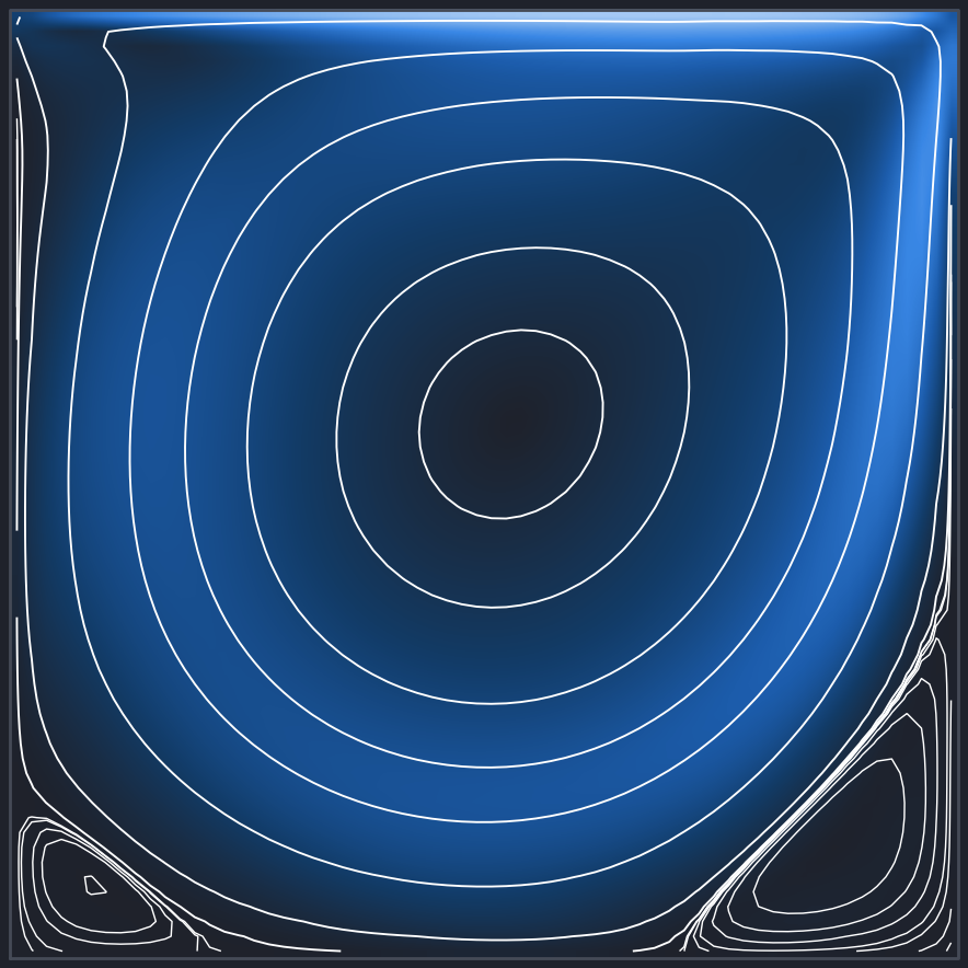
+y) moving right, the orientation of the reference data; the sample script below drives the -y face instead. Color shows the velocity magnitude, and lines are contours of the stream function. The primary vortex and the two secondary corner vortices are visible. See Validation for the comparison with reference data.The complete setup¤
import os
from lib.util.GPU_info import get_available_GPU_id
os.environ["CUDA_VISIBLE_DEVICES"] = str(get_available_GPU_id(active_mem_threshold=0.8, default=None))

import torch
cuda_device = torch.device("cuda")
dtype = torch.float32

import PISOtorch                  # core CUDA module
import PISOtorch_simulation       # helper for the PISO loop
import lib.data.shapes as shapes  # helpers for simple mesh generation
from lib.util.logging import setup_run, get_logger, close_logging

# logging and output: written to './test_runs/<time-stamp>_<name>/'
run_dir = setup_run("./test_runs", name="minimal-lid-sample_Re-1000_refine-1.1")
LOG = get_logger("Main")
stop_handler = PISOtorch_simulation.StopHandler(LOG)
stop_handler.register_signal()    # graceful shutdown with Ctrl-C

dims = 2
x, y = 32, 32                     # number of cells
viscosity = 1e-3                  # lid velocity 1 and cavity size 1 -> Re = 1000
velocity = 1
time_step = 0.25                  # the output time step
iterations = 100

# the mesh: corner vertices of all cells, refined towards all four walls
grid = shapes.make_wall_refined_ortho_grid(x, y, wall_refinement=["-x", "+x", "-y", "+y"], base=1.10)
grid = grid.cuda().contiguous()   # shape [1, 2, y+1, x+1]

# the domain holds global settings; the viscosity is a CPU tensor of shape [1]
domain = PISOtorch.Domain(dims, torch.tensor([viscosity], dtype=dtype), name="CavityDomain",
                          device=cuda_device, dtype=dtype, passiveScalarChannels=0)

# one block created from the mesh; fields and transformation metrics are created automatically
block = domain.CreateBlock(vertexCoordinates=grid, name="CavityBlock")

# blocks are periodic by default: close all faces (no-slip walls), then make one face the moving lid
block.CloseAllBoundaries()
lid_vel = torch.tensor([[velocity, 0]], device=domain.getDevice(), dtype=dtype)   # [1, dims]
block.CloseBoundary("-y", lid_vel)

domain.PrepareSolve()             # finalize the domain

sim = PISOtorch_simulation.Simulation(domain=domain,
    time_step=time_step,
    substeps="ADAPTIVE",          # split each output step to respect CFL <= 0.8
    corrector_steps=2,            # PISO default
    non_orthogonal=False,         # the mesh is orthogonal, no non-orthogonal correction needed
    pressure_tol=1e-5,
    velocity_corrector="FD",
    log_interval=1, norm_vel=True,
    output_resampling_shape=[x, y],   # also write images resampled to physical space
    log_dir=run_dir, save_domain_name="domain",
    stop_fn=stop_handler)

sim.run(iterations=iterations)

stop_handler.unregister_signal()
close_logging()
Run it from the repository root:
What happens¤
- Mesh.
make_wall_refined_ortho_gridreturns the corner vertices of a 32 × 32 grid. Neighboring cells grow by a factor of 1.10 away from the walls, so the boundary layers are resolved better. Boundary layers become thinner at higher Reynolds numbers. - Boundaries.
CloseAllBoundaries()turns the default periodic faces into no-slip walls.CloseBoundary("-y", lid_vel)then prescribes the lid velocity on one of them. A spatially varying lid velocity can be given as a tensor of shape[1, 2, 1, 32]. - Time stepping. Each of the 100 iterations advances the flow by 0.25 time units. With
"ADAPTIVE", every iteration is split into as many sub-steps as needed for a CFL number below 0.8. The log reports the count, e.g.Adaptive time step 2.500e-01 (CFL=0.80) used 23 substeps. - Output. At every iteration, the log lists the velocity, pressure and divergence statistics, and velocity (
v_*.png) and pressure (p_*.png) images are written. The-rvariants are resampled to physical space. At the end, the domain is saved asdomain.json/domain.npz.
The 3D version¤
minimal_lid_sample3D.py makes three changes: it uses dims = 3, it extrudes the 2D mesh in z, and it gives the lid velocity three components:
dims = 3
grid = shapes.make_wall_refined_ortho_grid(x, y, wall_refinement=["-x", "+x", "-y", "+y"], base=1.10)
grid = shapes.extrude_grid_z(grid, z, 0, 2)          # 32 cells in z, from z=0 to z=2
...
lid_vel = torch.tensor([[velocity, 0, 0]], device=domain.getDevice(), dtype=dtype)
For 3D output, the images show slices, and log_vtk=True writes VTK files for ParaView.
Variations to try¤
- Reynolds number. Lower
viscosity(and increase the resolution and refinement) for higher Reynolds numbers. The paper validates Re = 100 and 5000 in 2D and Re = 1000 in 3D. - Double precision. Set
dtype = torch.float64for tighter solver tolerances (default 1e-8 instead of 1e-5). - Moving walls. Close other faces with tangential velocities.
- Passive scalar. Set
passiveScalarChannels=1and initializeblock.passiveScalarto watch a dye being mixed.