Learning a Forcing¤
Source
- Script:
learning_sample.py - Run:
python learning_sample.pyfrom the repository root
This is the smallest end-to-end example of learning through the differentiable solver. A periodic 2D channel is driven by an unknown forcing. Given a target simulation, the goal is to recover the forcing in two ways:
- Direct optimization: a constant forcing vector is optimized with gradient descent.
- Network training: a small CNN learns to predict the forcing from the velocity field in every simulation step.
Setup¤
def make_forcing_domain(x: int, y: int, viscosity: float = 1, dtype=torch.float32):
    domain = PISOtorch.Domain(2, torch.tensor([viscosity], dtype=dtype), name="DomainForcingSample",
                              dtype=dtype, device=cuda_device)
    # without a mesh, a block is created from its resolution and has unit cell size
    block = domain.CreateBlockWithSize(PISOtorch.Int4(x=x, y=y), name="Block")
    # blocks are periodic by default; closing -y also closes +y -> periodic channel in x
    block.CloseBoundary("-y")
    domain.PrepareSolve()
    return domain
The target is a clone of this domain, simulated for 3 steps with the forcing \((1, 0)\):
target_domain = domain.Clone()                 # deep copy, independent tensors
target_domain.PrepareSolve()
target_domain.getBlock(0).setVelocitySource(torch.tensor([[1, 0]], dtype=dtype, device=cuda_device))
target_domain.UpdateDomainData()
PISOtorch_simulation.Simulation(target_domain, substeps=1, time_step=0.1, non_orthogonal=False,
                                log_images=False).run(3)   # the sample writes images to a log_dir instead
1. Optimizing a constant forcing¤
var_forcing = torch.zeros([1, 2], device=cuda_device, dtype=dtype, requires_grad=True)
optimizer = torch.optim.SGD([var_forcing], lr=1e-2, momentum=0)

for opt_step in range(opt_steps):
    opt_domain = domain.Copy()                 # shares tensors with `domain`; safe in differentiable mode
    opt_domain.getBlock(0).setVelocitySource(var_forcing)
    opt_domain.PrepareSolve()

    sim = PISOtorch_simulation.Simulation(opt_domain, substeps=1, time_step=0.1,
                                          non_orthogonal=False, differentiable=True,
                                          log_images=False)
    sim.run(3, log_domain=False)

    loss = sum(torch.sum((b.velocity - t.velocity) ** 2)
               for b, t in zip(opt_domain.getBlocks(), target_domain.getBlocks()))
    loss.backward()
    optimizer.step()
    optimizer.zero_grad()
    opt_domain.Detach()                        # break the cycle between domain and autograd graph
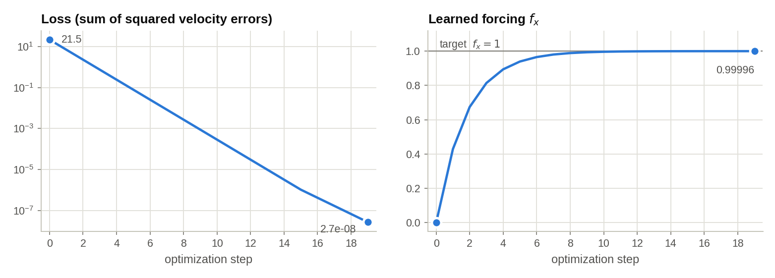
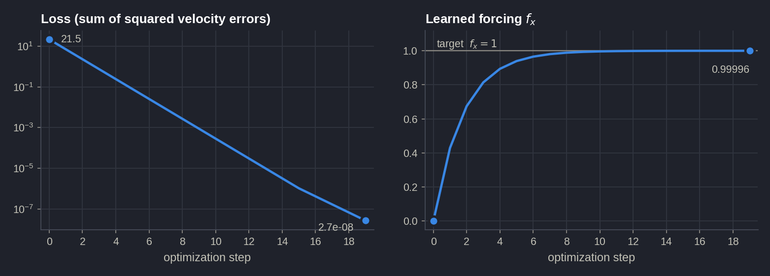
The gradient \(\partial L/\partial \mathbf{f}\) is computed by backpropagating through all three PISO steps: the advection–diffusion matrix and right-hand-side setup, the BiCGStab solves (adjoint solves with \(C^\mathsf{T}\)), the pressure setup, the CG solves and the velocity corrections.
2. Training a forcing network¤
The sample's network is deliberately tiny. It consists of 1×1 convolutions, so it acts per cell:
class ForcingNet(torch.nn.Module):
    def __init__(self):
        super().__init__()
        self.conv1 = torch.nn.Conv2d(2, 8, 1, 1)
        self.conv2 = torch.nn.Conv2d(8, 4, 1, 1)
        self.conv3 = torch.nn.Conv2d(4, 2, 1, 1)

    def forward(self, x):
        x = torch.nn.functional.relu(self.conv1(x))
        x = torch.nn.functional.relu(self.conv2(x))
        return self.conv3(x)
Instead of setting a constant source, a PRE callback evaluates the network on the current velocity at the start of every PISO step. The gradient therefore also flows through the network's influence on later steps:
forcing_net = ForcingNet().to(cuda_device)
optimizer = torch.optim.Adam(forcing_net.parameters(), lr=4e-4)

def pfn_set_forcing(domain, time_step, **kwargs):
    domain.getBlock(0).setVelocitySource(forcing_net(domain.getBlock(0).velocity))
    domain.UpdateDomainData()

prep_fn = {}
PISOtorch_simulation.append_prep_fn(prep_fn, "PRE", pfn_set_forcing)
# ... same loop as above, with Simulation(..., prep_fn=prep_fn, differentiable=True)
Running¤
The script runs both variants: 10 gradient-descent steps for the constant forcing and 100 Adam steps for the network. For each, it writes opt_stats.pdf with the loss curve, the learned forcing (forcing.npz) or network weights (forcingNet.pt), and images of the first and last optimization step. Increase opt_steps to train the network further.
This pattern of a network that is evaluated in a callback, a differentiable unroll, a loss and Detach() scales directly to the large learning setups of the paper, such as the Turbulent Channel Flow SGS Model.